Quick Start

A pangenome models the full set of genomic elements in a given species or clade. It can efficiently be encoded in the form of a variation graph, a type of sequence graph that embeds the linear sequences as paths in the graphs themselves.

To exchange pangenomes, the community frequently uses a strict subset of the Graphical Fragment Assembly GFA format version 1 (GFAv1).

In the following, a generic quick start guide for the pggb pipeline is described. The input is a FASTA file (e.g. input.fa) containing all sequences to build a pangenome graph from.

Step 1 - Sequence Preparation

Put your sequences in one FASTA file in.fa, optioanlli compress it with bgzip, and index it with samtools faidx in.fa (or samtools faidx in.fa.gz for compressed input). If you have many samples and/or haplotypes, we suggest using the PanSN-spec naming pattern.

Step 2 - Sequence partitioning (OPTIONAL)

If you have whole-genome assemblies, you might consider partitioning your sequences into communities, which usually correspond to the different chromosomes of the genomes. Then, you can run pggb on each community (set of sequences) independently (see partition before pggb).

Step 3 - Graph Building

To build a graph from a 9-haplotype in.fa, in the directory output, scaffolding the graph using 5kb matches at >= 90% identity, and using 16 parallel threads for processing, execute:

pggb \
-i in.fa \       # input file in FASTA format
-o output \      # output directory
-n 9  \          # number of haplotypes (optional with PanSN-spec)
-t 16            # number of threads (defaults to ``getconf _NPROCESSORS_ONLN``)
-p 90 \          # (default) minimum average nucleotide identity for a seed mapping
-s 5000 \        # (default) segment length
-V 'ref:1000'    # make a VCF against "ref" decomposing variants >1000bp

The final process output will be called outdir/input.fa*smooth.fix.gfa. By default, we render 1D and 2D visualizations of the graph with odgi, which are very useful to understand the result of the build.

partition before pggb

In the above example, to partition your sequences into communities, execute:

partition-before-pggb -i in.fa \       # input file in FASTA format
                      -o output \      # output directory
                      -n 9 \           # number of haplotypes (optional with PanSN-spec)
                      -t 16 \          # number of threads
                      -p 90 \          # minimum average nucleotide identity for segments
                      -s 5k \          # segment length for scaffolding the graph
                      -V 'ref:1000'    # make a VCF against "ref" decomposing variants >1000bp

This generates the command lines to run pggb on each community (2 in this example) independently:

pggb -i output/in.fa.dd9e519.community.0.fa \
     -o output/in.fa.dd9e519.community.0.fa.out \
     -p 5k -l 25000 -p 90 -n 9 -K 19 -F 0.001 \
     -k 19 -f 0 -B 10000000 \
     -H 9 -j 0 -e 0 -G 700,900,1100 -P 1,19,39,3,81,1 -O 0.001 -d 100 -Q Consensus_ \
     -V ref:1000 --threads 16 --poa-threads 16
pggb -i output/in.fa.dd9e519.community.1.fa \
     -o output/in.fa.dd9e519.community.1.fa.out \
     -p 5k -l 25000 -p 90 -n 9 -K 19 -F 0.001 \
     -k 19 -f 0 -B 10000000 \
     -H 9 -j 0 -e 0 -G 700,900,1100 -P 1,19,39,3,81,1 -O 0.001 -d 100 -Q Consensus_ \
     -V ref:1000 --threads 16 --poa-threads 16

See also the Sequence partitioning tutorial for more information.

Example - Building an MHC Pangenome Graph

We build a MHC class II ALTs GRCh38 pangenome graph from 10 haplotypes using test data from this repository's data/HLA directory.

git clone --recursive https://github.com/pangenome/pggb
cd pggb
./pggb -i data/HLA/DRB1-3123.fa.gz -p 70 -s 3000 -n 10 -t 16 -V 'gi|568815561' -o out

This writes to directory out: a variation graph in GFA format, a multiple sequence alignment in MAF format, and several diagnostic images. By default, the outputs are named according to the input file and a hash of the construction parameters. Adding -v prohibits the rendering of 1D and 2D diagnostic images of the graph. This can reduce running time, because the calculation of the 2D layout can take a while. By default, redundant structures in the graph are collapsed by applying GFAffix. We also call variants with -V with respect to the reference gi|568815561.

1D Graph Visualization

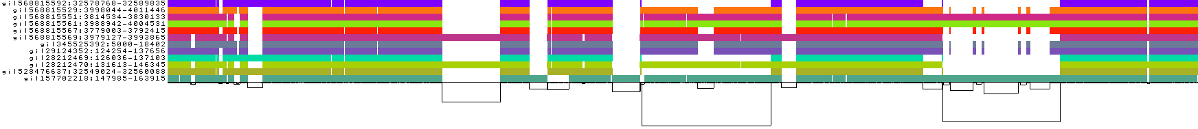
Explanation of this 1D visualization:

• The graph nodes are arranged from left to right forming the pangenome sequence.

• The colored bars represent the binned, linearized renderings of the embedded paths versus this pangenome sequence in a binary matrix.

• The path names are visualized on the left.

• The black lines under the paths, so called links, represent the topology of the graph.

2D Graph Visualization

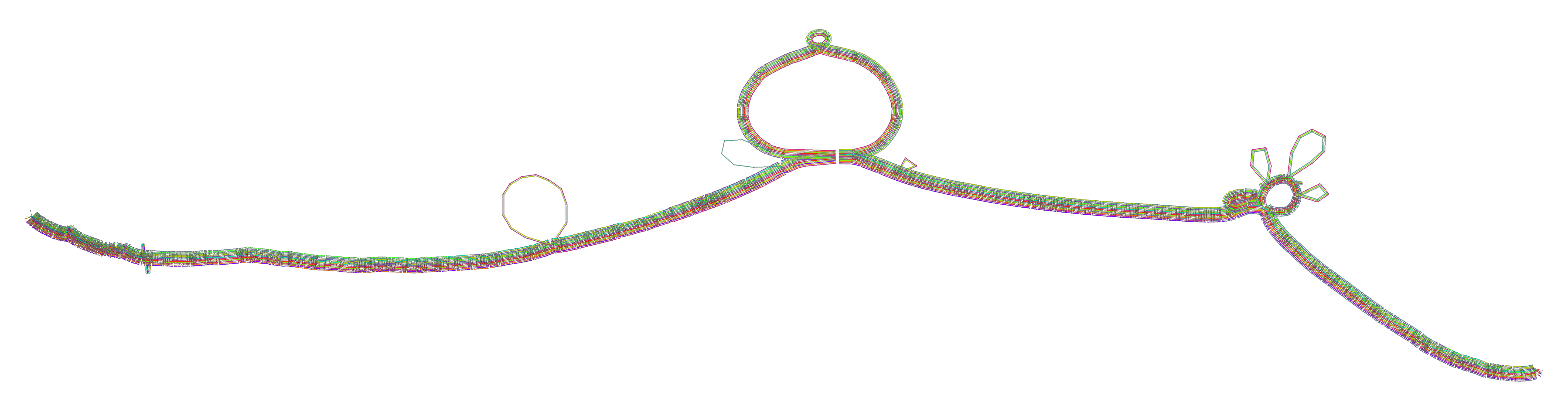
Explanation of this 2D visualization:

• Each colored rectangle represents a node of a path. The node’s x-coordinates are on the x-axis and the y-coordinates are on the y-axis, respectively.

• A bubble indicates that here some paths have a diverging sequence or it can represent a repeat region.

For more information about the layout, please visit https://odgi.readthedocs.io/en/latest/rst/tutorials/sort_layout.html.