Sequence partitioning
Author: Andrea Guarracino
Synopsis
Pangenome graphs can represent all mutual alignments of collections of sequences. However, we can't really expect to pairwise map all sequences together and obtain well separated connected components. It is likely to get a giant connected component, and probably a few smaller ones, due to incorrect mappings or false homologies. This might unnecessarily increase the computational burden, as well as complicate the downstream analyzes. Therefore, it is recommended to split up the input sequences into communities in order to find the latent structure of their mutual relationship. For example, the communities can represent the different chromosomes of the input genomes.
Warning
If you know in advance that your sequences present particular rearrangements (like rare chromosome translocations), you might consider skipping this step or tuning it accordingly to your biological questions.
Steps
Here we show how to detect the communities of 7 Saccharomyces cerevisiae assemblies (Yue et al., 2016) from the Yeast Population Reference Panel (YPRP).
Install the dependencies
We applies the Leiden algorithm (Trag et al., 2018) implemented in
the leidenalg package:
pip3 install python-igraph
pip3 install pycairo # Only needed for visualization
Download the assemblies
Assuming that your current working directory is the root of the pggb repository, to download the YPRP panel,
execute:
mkdir -p assemblies/yprp_panel
cd assemblies/yprp_panel
cat ../../docs/data/scerevisiae.yprp.urls | parallel -j 4 'wget -q {} && echo got {}'
For each sample, to put genome and mitochondrial sequences together, execute:
ls *.fa.gz | cut -f 1 -d '.' | uniq | while read f; do
    echo $f
    zcat $f.* > $f.fa
done
Pangenome Sequence Naming
To change the sequence names according to PanSN-spec, we use fastix:
ls *.fa | while read f; do
    sample_name=$(echo $f | cut -f 1 -d '.');
    echo ${sample_name}
    fastix -p "${sample_name}#1#" $f >> scerevisiae7.fasta
done
bgzip -@ 4 scerevisiae7.fasta
samtools faidx scerevisiae7.fasta.gz
We specify haplotype_id equals to 1 for all the assemblies, as they are all haploid.
Community detection
We need to obtain the mutual relationship between the input assemblies in order to detect the underlying communities. To compute the pairwise mappings with wfmash, execute:
wfmash scerevisiae7.fasta.gz -p 90 -n 6 -t 4 -m > scerevisiae7.mapping.paf
We set -p 90 as we expect a sequence divergence of ~10% between these assemblies (see the Divergence estimation
tutorial for more information), while -n 6 indicates the number of mappings to keep for each homologous region
identified, set as the number of haplotypes (number of haploid samples in this example) minus 1.
To project the PAF mappings into a network format (an edge list), execute:
python3 ../../scripts/paf2net.py -p scerevisiae7.mapping.paf
The paf2net.py script creates 3 files:
scerevisiae7.mapping.paf.edges.list.txtis the edge list representing the pairs of sequences mapped in the PAF;scerevisiae7.mapping.paf.edges.weights.txtis a list of edge weights (long and high estimated identity mappings have greater weight);scerevisiae7.mapping.paf.vertices.id2name.txtis the 'id to sequence name' map.
To identity the communities, execute:
python3 ../../scripts/net2communities.py \
    -e scerevisiae7.mapping.paf.edges.list.txt \
    -w scerevisiae7.mapping.paf.edges.weights.txt \
    -n scerevisiae7.mapping.paf.vertices.id2name.txt
The paf2net.py script creates a set of *.community.*.txt files one for each of the 15 communities detected.
Each txt file lists the sequences that belong to the same community. For example, to see the sequences in one community,
execute:
cat scerevisiae7.mapping.paf.edges.weights.txt.community.6.txt
DBVPG6044#1#chrVII
S288C#1#chrVII
SK1#1#chrVII
Y12#1#chrVII
YPS128#1#chrVII
DBVPG6044#1#chrVIII
S288C#1#chrVIII
SK1#1#chrVIII
UWOPS034614#1#chrVII
UWOPS034614#1#chrVIII
Y12#1#chrVIII
YPS128#1#chrVIII
DBVPG6765#1#chrVII
DBVPG6765#1#chrVIII
This community presents both chrVII and chrVIII contigs. This is one of structural rearrangements known for these samples (Yue et al., 2016). To see the chromosome content of each community, execute:
seq 0 14 | while read i; do
    chromosomes=$(cat scerevisiae7.mapping.paf.edges.weights.txt.community.$i.txt | cut -f 3 -d '#' | sort | uniq | tr '\n' ' ');
    echo "community $i --> $chromosomes";
done
community 0 --> chrI
community 1 --> chrII
community 2 --> chrIII
community 3 --> chrIV
community 4 --> chrV
community 5 --> chrVI
community 6 --> chrVII chrVIII
community 7 --> chrIX
community 8 --> chrX chrXIII
community 9 --> chrXI
community 10 --> chrXII
community 11 --> chrXIV
community 12 --> chrXV
community 13 --> chrXVI
community 14 --> chrMT
The paf2net.py script can also generate a visualization of the communities detected. To request such a visualization,
run the script by specifying the --plot flag (it can be slow with big datasets):
python3 ../../scripts/net2communities.py \
    -e scerevisiae7.mapping.paf.edges.list.txt \
    -w scerevisiae7.mapping.paf.edges.weights.txt \
    -n scerevisiae7.mapping.paf.vertices.id2name.txt \
    --plot
The visualization is written in the scerevisiae7.mapping.paf.edges.list.txt.communities.pdf file.
Here is the visualization of the two communities that depict the structural rearrangements (in grey and green):
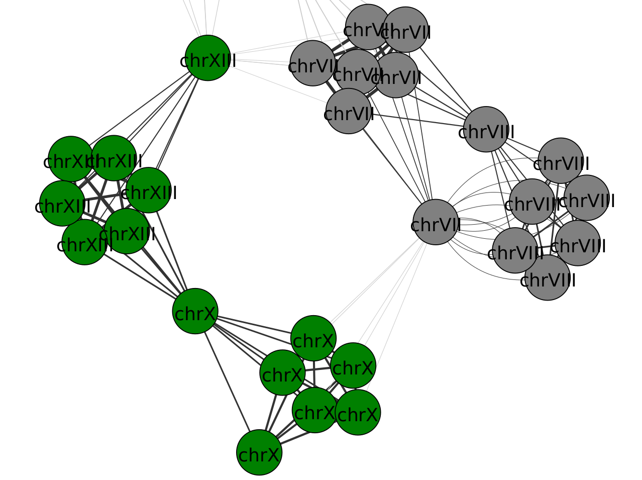
Vertices represent the contigs, colored by community. Arrows represent the mappings between contigs: the black ones indicate mappings between contig of the same community, while gray indicates links between different communities.
Data partitioning
Each community can be managed by pggb independently of the others. To partition the communities, execute:
seq 0 14 | while read i; do
    echo "community $i"
    samtools faidx scerevisiae7.fasta.gz $(cat scerevisiae7.mapping.paf.edges.weights.txt.community.$i.txt) | \
    bgzip -@ 4 -c > scerevisiae7.community.$i.fa.gz
    samtools faidx scerevisiae7.community.$i.fa.gz
done
All scerevisiae7.community.*.fa.gz files are ready to be processed separately with pggb.
Note
If you need to join all pggb's partitioned graphs again, you can use odgi squeeze (see its documentation).
Mash-based partitioning
To obtain the reciprocal relationship between the input sets of sequences, in order to identify the underlying communities, we can also use mash. The main advantage of such an approach is that it allows us not to have to specify an initial level of expected identity.
To compute the pairwise distances between all pairs of input sequences, execute:
mash dist scerevisiae7.fasta.gz scerevisiae7.fasta.gz -s 10000 -i > scerevisiae7.distances.tsv
The mash dist command estimates the distance of each pair of sequences in input.
The -s 10000 specifies a bigger sketch size for each sequence to compare: a higher value allows for more accurate estimates
(see here how the distance estimation works).
Moreover, -i indicates to compare the individual sequences in input, and not the FASTA files as a whole.
To visualize the first rows of the scerevisiae7.distances.tsv file, execute:
head -n 5 scerevisiae7.distances.tsv | column -t
DBVPG6044#1#chrI    DBVPG6044#1#chrI  0         0             10000/10000
DBVPG6044#1#chrII   DBVPG6044#1#chrI  0.184461  0             105/10000
DBVPG6044#1#chrIII  DBVPG6044#1#chrI  0.186761  0             100/10000
DBVPG6044#1#chrIV   DBVPG6044#1#chrI  0.220489  1.83465e-228  49/10000
DBVPG6044#1#chrV    DBVPG6044#1#chrI  0.176252  0             125/10000
The result is a tab-separated file, with each row reporting the names of the compared sequences, their mash-distance,
the P-value associated with the mash-distance, and the ratio of the number of shared hashes divided by the number of
hashes considered (set to 10000 with -s 10000).
To project the distances into a network format (an edge list), and then identify the communities, execute:
python3 ../../scripts/mash2net.py -m scerevisiae7.distances.tsv

python3 ../../scripts/net2communities.py \
    -e scerevisiae7.distances.tsv.edges.list.txt \
    -w scerevisiae7.distances.tsv.edges.weights.txt \
    -n scerevisiae7.distances.tsv.vertices.id2name.txt

seq 0 14 | while read i; do
    chromosomes=$(cat scerevisiae7.distances.tsv.edges.weights.txt.community.$i.txt | cut -f 3 -d '#' | sort | uniq | tr '\n' ' ');
    echo "community $i --> $chromosomes";
done
community 0 --> chrII
community 1 --> chrI
community 2 --> chrIII
community 3 --> chrIV
community 4 --> chrV
community 5 --> chrVI
community 6 --> chrVII chrVIII
community 7 --> chrIX
community 8 --> chrX chrXIII
community 9 --> chrXI
community 10 --> chrXII
community 11 --> chrXIV
community 12 --> chrXV
community 13 --> chrXVI
community 14 --> chrMT