Small variants evaluation

Author: Andrea Guarracino

Synopsis

The major histocompatibility complex (MHC) is a large locus in vertebrate DNA containing a set of closely linked polymorphic genes that code for cell surface proteins essential for the adaptive immune system. In humans, the MHC region occurs on chromosome 6.

Steps

Data collection

We map HPRC chromosome 6 contigs to the MHC ALT haplotypes from GRCh38:

wfmash -t 16 -m -s 5000 -p 98 MHC.fa.gz chr6.pan.fa > HPRCy1.pan.chr6_vs_MHC.paf

Then, we make a BED file for the mappings and merge the regions in it to make a single BED record per matching contig:

awk '{ print $1, $3, $4 }' HPRCy1.pan.chr6_vs_MHC.paf | tr ' ' '\t' | sort -V > HPRCy1.MHC.bed
bedtools merge -d 1000000 -i HPRCy1.MHC.bed > HPRCy1.MHC.merge.bed

Finally, we extract the FASTA file for the regions:

bedtools getfasta -fi /lizardfs/erikg/HPRC/year1/parts/chr6.pan+refs.fa -bed HPRCy1.MHC.merge.bed | bgzip -c -@ 16 > HPRCy1.MHC.fa.gz
samtools faidx HPRCy1.MHC.fa.gz

Pangenome Sequence Naming

Contigs already respect the Pangenome Sequence Naming specification (PanSN-spec).

cut -f 1 HPRCy1.MHC.fa.gz.fai | head -n 6

HG00438#1#JAHBCB010000040.1:22870000-27725000
HG00438#2#JAHBCA010000042.1:22875000-27895000
HG00621#1#JAHBCD010000020.1:22865000-27905000
HG00621#2#JAHBCC010000005.1:28460000-33400000
HG00673#1#JAHBBZ010000030.1:28480000-33310000
HG00673#2#JAHBBY010000018.1:0-2900000

Divergence estimation

The human MHC locus presents a high sequence divergence, so we will set the mapping identity (-p parameter) in pggb to 95.

Sequence partitioning

As the dataset is small, we do not need to partition sequences (see the Sequence partitioning tutorial for more information).

Pangenome graph building

To build the MHC pangenome graph, execute:

pggb -i HPRCy1.MHC.fa.gz -p 95 -n 90 -t 16 -G 13117,13219 -o HPRCy1.MHC.s10k.p95.output

Graph statistics

To collect basic graph statistics, execute:

odgi stats -i HPRCy1.MHC.s10k.p95.output/*.final.gfa -t 16 -S

#length     nodes   edges   paths
5315371     309186  429323  126

Identify variants with vg

To call variants for each contig, execute:

vg deconstruct -P chm13 -H '?' -e -a -t 48 HPRCy1.MHC.s10k.p95.output/HPRCy1.MHC.fa.gz.39ffa23.e34d4cd.be6be64.smooth.final.gfa | \
    bgzip -c -@ 16 > HPRCy1.MHC.s10k.p95.output/HPRCy1.MHC.fa.gz.39ffa23.e34d4cd.be6be64.smooth.final.chm13.vcf.gz

-H '?' avoids managing the path name hierarchy when calling variants, then emitting variants for each contig.

To filter variants (by using nesting information from the pangenome graph) and realign reference and alternate alleles, execute:

vcfbub -l 0 -a 100000 --input HPRCy1.MHC.s10k.p95.output/HPRCy1.MHC.fa.gz.39ffa23.e34d4cd.be6be64.smooth.final.chm13.vcf.gz | \
    vcfwave -I 1000 -t 48 | bgzip -@ 16 \
    > HPRCy1.MHC.s10k.p95.output/HPRCy1.MHC.fa.gz.39ffa23.e34d4cd.be6be64.smooth.final.chm13.vcfbub.a100k.wave.vcf.gz

Take SNPs from the PGGB VCF file:

REF=chm13#chr6:28380000-33300000.fa
NAMEREF=chm13

cut -f 1 HPRCy1.MHC.fa.gz.fai | grep chm13 -v | while read CONTIG; do
    echo $CONTIG

    bash vcf_preprocess.sh \
        HPRCy1.MHC.s10k.p95.output/*.vcfbub.a100k.wave.vcf.gz \
        $CONTIG \
        1 \
        $REF
done

Identify variants with nucmer

Prepare the reference FASTA file:

samtools faidx HPRCy1.MHC.fa.gz chm13#chr6:28380000-33300000 > chm13#chr6:28380000-33300000.fa

Align each sequence against the reference with nucmer:

REF=chm13#chr6:28380000-33300000.fa
NAMEREF=chm13

mkdir -p nucmer/

cut -f 1 HPRCy1.MHC.fa.gz.fai | grep chm13 -v | while read CONTIG; do
    echo $CONTIG

    PREFIX=nucmer/${CONTIG}_vs_${NAMEREF}
    samtools faidx HPRCy1.MHC.fa.gz $CONTIG > $CONTIG.fa

    nucmer $REF $CONTIG.fa --prefix "$PREFIX"

    show-snps -THC "$PREFIX".delta > "$PREFIX".var.txt

    rm $CONTIG.fa
done

Using the nucmer2vcf.R script, generate VCF files for each sequence with respect to the reference with nucmer:

REF=chm13#chr6:28380000-33300000.fa
NAMEREF=chm13

NUCMER_VERSION="4.0.0beta2"
cut -f 1 HPRCy1.MHC.fa.gz.fai | grep chm13 -v | while read CONTIG; do
    echo $CONTIG

    PREFIX=nucmer/${CONTIG}_vs_${NAMEREF}
    Rscript nucmer2vcf.R "$PREFIX".var.txt $CONTIG $REF $NUCMER_VERSION $PREFIX.vcf
    bgzip -@ 16 $PREFIX.vcf
    tabix $PREFIX.vcf.gz
done

Variants evaluation

Prepare the reference in SDF format for variant evaluation with rtg vcfeval:

rtg format -o chm13#chr6:28380000-33300000.sdf chm13#chr6:28380000-33300000.fa

Compare nucmer-based SNPs with PGGB-based SNPs:

REFSDF=chm13#chr6:28380000-33300000.sdf
NAMEREF=chm13

cut -f 1 HPRCy1.MHC.fa.gz.fai | grep chm13 -v | while read CONTIG; do
    echo $CONTIG

    PREFIX=nucmer/${CONTIG}_vs_${NAMEREF}

    PATH_PGGB_VCF=HPRCy1.MHC.s10k.p95.output/HPRCy1.MHC.fa.gz.*.smooth.final.chm13.vcfbub.a100k.wave.${CONTIG}.max1.vcf.gz

    # Merge regions closer than 1000 bps to define the callable regions where to evaluate the variants
    dist=1000

    rtg vcfeval \
        -t $REFSDF \
        -b $PREFIX.vcf.gz \
        -c $PATH_PGGB_VCF \
        -T 16 \
        -e <(bedtools intersect -a <(bedtools merge -d $dist -i $PREFIX.vcf.gz ) -b <(bedtools merge -d $dist -i $PATH_PGGB_VCF)) \
        -o vcfeval/${CONTIG}
done

Collect statistics:

cd vcfeval
(echo contig precision recall f1.score; grep None */*txt | sed 's,/summary.txt:,,' | tr -s ' ' | cut -f 1,7,8,9 -d ' ' ) | tr ' ' '\t' > statistics.tsv

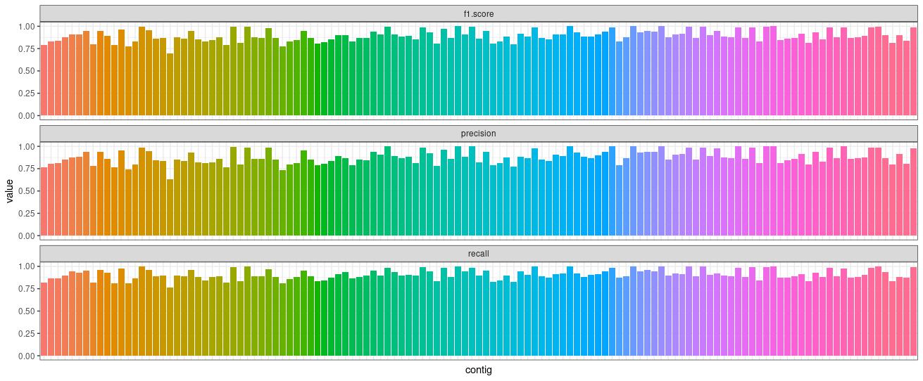
Plot statistics:

require(ggplot2)
require(tidyr)

stat_df <- read.table('statistics.tsv', sep = '\t', header = T, comment.char = '?')

stat_df <- pivot_longer(stat_df,precision:f1.score,"Metric")

ggplot(stat_df,aes(x=contig,y=value,fill=contig))+
  geom_bar(stat="identity") +
  facet_wrap(~Metric, ncol = 1)+
  theme_bw() +
  theme(
    axis.ticks.x = element_blank(),
    axis.text.x = element_blank()
  ) +
  theme(legend.position="none")